2025-09-21
4. Transforming, Scaling, and Fitting the Data
2025-09-21
Methodology
Because our target variable, HP, is a continuous numerical value, we will be using a regression model to predict it. And because we have a large number of features with many that do not have high correlation with our target variable, we can use Lasso Regression for its ability to perform feature selection and regularization. However, we can also see from our correlation heatmap that there are some features that have high correlation with each other which can lead to multicollinearity issues. To address this, we will use elastic net with provide a balance between Lasso and Ridge regression.
Feature Selection
Now we need to prepare our feature set. Based on our exploratory data
analysis, I decided to drop total_resistance_multiplier since it had
very little variation and didn’t correlate well with HP. We also need to
handle any missing text values by filling them with empty strings.
from sklearn.linear_model import ElasticNetCV
from sklearn.model_selection import train_test_split
from sklearn.preprocessing import StandardScaler, FunctionTransformer
from sklearn.compose import ColumnTransformer
from sklearn.pipeline import Pipeline, FeatureUnion
from sklearn.metrics import root_mean_squared_error, mean_absolute_error, r2_score
from sklearn.impute import SimpleImputer
from sklearn.decomposition import PCA
from sklearn.cluster import KMeans

df = pd.read_csv('data/first_gen_pokemon_final_features.csv')
df.drop(columns=['id', 'flavorText', 'reasoning', 'ability_name', 'attack_name'], inplace=True)

target = 'hp'
y = df[target]

cols_to_drop = [
  'hp', 'total_resistance_multiplier'
]
X = df.drop(columns=cols_to_drop)
Categorizing Features by Type
Different types of features need different preprocessing steps. Lets organize our features into three categories: numeric features (need scaling), text features (need TF-IDF vectorization), and binary features (can be used as-is).
numeric_features = [
    'level', 'convertedRetreatCost', 'number', 'primary_pokedex_number',
    'pokemon_count', 'total_weakness_multiplier', 'total_weakness_modifier',
    'total_resistance_modifier', 'pokedex_frequency', 'artist_frequency',
    'ability_count', 'attack_count', 'base_damage', 'attack_cost',
    'attack_damage', 'attack_utility', 'ability_damage', 'ability_utility',
  'text_depth', 'word_count', 'keyword_score'
]

binary_features = [
    col for col in X.columns if col not in numeric_features
]

print(f"Numeric features: {len(numeric_features)}")
print(f"Binary features: {len(binary_features)}")
Numeric features: 21
Binary features: 93We can see that we have 14 numeric features, 2 text features, and many binary features (mostly from our one-hot encoding in our feature engineering step).
Train-Test Split
Before we do any transformations, we need to split our data into training and testing sets. This ensures we don’t leak information from the test set into our model. I’m using a 80/20 split with a random state for reproducibility.
X_train, X_test, y_train, y_test = train_test_split(X, y, test_size=0.5, random_state=123)Building the Preprocessing Pipeline
Now comes the important part - setting up our preprocessing pipeline. We need to:
- Numeric features: Impute missing values with the median, then standardize (scale to mean=0, std=1)
- Binary features: Pass through unchanged since they’re already in the right format
- Text features: Convert to TF-IDF vectors with a maximum of 100 features each
We’ll use scikit-learn’s ColumnTransformer to apply different
preprocessing steps to different feature types, and then combine
everything with a Ridge regression model in a single pipeline.
Additionally we will be using ElasticNetCV which performs
cross-validated elastic net regression to find the optimal
hyperparameters for our model. This requires us to set up a grid of
alpha and l1_ratio values to search over.
numeric_pipeline = Pipeline(steps=[
  ('impute', SimpleImputer(strategy='median')),
  ('scale', StandardScaler()),
])

preprocessor = ColumnTransformer(
    transformers=[
        ('numeric', numeric_pipeline, numeric_features),
        ('pass', 'passthrough', binary_features),
    ],
    remainder='drop'
)

l1_ratios = [0.1, 0.5, 0.7, 0.9, 0.95, 0.99, 1.0]

model_pipeline = Pipeline(steps=[
  ('preprocessor', preprocessor),
  ('model', ElasticNetCV(l1_ratio=l1_ratios, cv=5, random_state=123))
])

model_pipeline.fit(X_train, y_train)
y_pred = model_pipeline.predict(X_test)
Results
After training our elastic net regression model, we can evaluate how many features were selected (non-zero coefficients) and the model’s performance on the test set. We see that out of the 114 features we started with, we dropped 48 features, leaving us with 66 features that the model found useful for predicting HP. This could mean a few things: some features may be redundant, some may not have a strong relationship with HP, or the model may be prioritizing simpler explanations.
final_model = model_pipeline.named_steps['model']

feature_names = numeric_features + binary_features

import pandas as pd
coef_df = pd.DataFrame({
    'Feature': feature_names,
    'Coefficient': final_model.coef_
})

dropped_features = coef_df[coef_df['Coefficient'] == 0]
print(f"Total features: {len(feature_names)}")
print(f"Features dropped (Noise): {len(dropped_features)}")
Total features: 114
Features dropped (Noise): 48Evaluating the model’s performance on the test set, we achieved an R² score of 0.936 and an RMSE of 15.50. An R² score of 0.936 indicates that our model explains a significant portion of the variance in HP, which is quite good. The RMSE of 15.50 means that, on average, our predictions are off by about 15.5 HP points.
rmse = root_mean_squared_error(y_test, y_pred)
print(f"RMSE: {rmse:.2f} hp")

mae = mean_absolute_error(y_test, y_pred)
print(f"MAE: {mae:.2f} hp")

r2 = r2_score(y_test, y_pred)
print(f"R-Squared: {r2:.3f}")
RMSE: 15.50 hp
MAE: 11.51 hp
R-Squared: 0.936Finally, we can plot the predicted vs actual HP values to visually assess the model’s performance. Ideally, we want the points to fall along the diagonal line, indicating perfect predictions. We can see that most points are close to the line, but there are some deviations, especially for mid-range and high HP values. This suggests that while the model performs well overall, there may be room for improvement in predicting certain HP ranges.
import matplotlib.pyplot as plt
import seaborn as sns

plt.figure(figsize=(8, 8))
sns.scatterplot(x=y_test, y=y_pred)
plt.xlabel("Actual HP (y_test)")
plt.ylabel("Predicted HP (y_pred)")
plt.title("Actual vs. Predicted HP")

plt.plot([y_test.min(), y_test.max()], [y_test.min(), y_test.max()], 'r--', lw=2)
plt.show()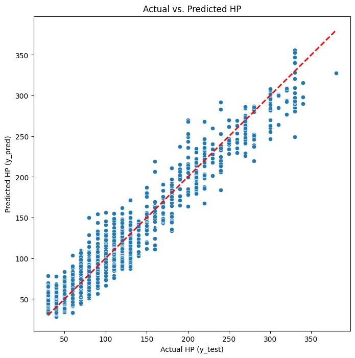
Discussion and Conclusion
Overall, our elastic net regression model performed well in predicting the HP of Pokemon cards based on various features. The high R² score and low RMSE indicate that the model was able to capture the underlying patterns in the data. The feature selection process also helped reduce the complexity of the model by eliminating less important features. However, there are still areas for improvement. The deviations in the predicted vs actual plot suggest that the model may struggle with certain HP ranges, particularly mid-range and high HP values. Future work could involve exploring more advanced modeling techniques.